It's no secret to project managers worldwide that optimizing value delivery is paramount. Having a well-defined, straightforward, and predictable work process is mayhem, yet very few managers are aware of Little's law. There are several reasons for this. One is the lack of comprehensive examples that explain the law, and another is that, in a way, it contradicts the idea "the more I start, the more I will get done”.
That’s why, in this article, you’ll learn:
- What is Little’s law and its origins
- How to calculate the theorem
- What are its benefits and applications
What Is Little's Law?
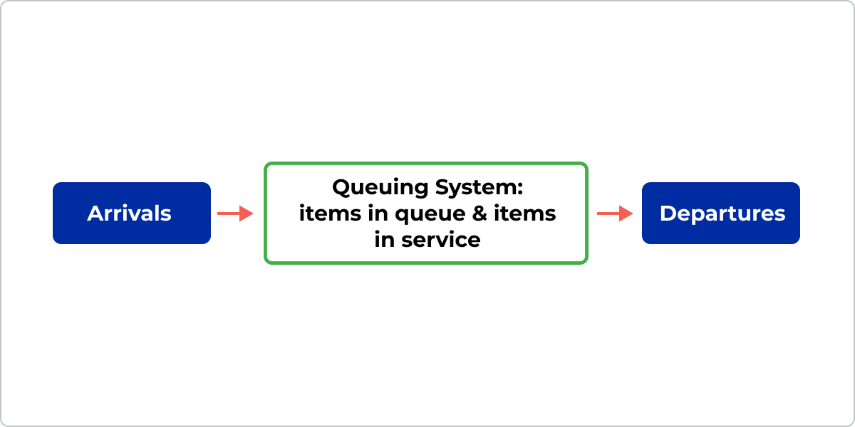
Little's law is a fundamental theorem in queuing theory that provides a simple but powerful relationship between three primary characteristics of a queuing system, namely:
- L = the average number of items in a queuing system
- λ = the average number of items arriving at the system per unit of time
- W = the average waiting time an item spends in a queuing system
Little’s law is formulated as: L=λW
The formula states that the average number of items in the system equals the product of their average arrival rate and the average time an item spends in the system.

How items flow in a queuing system
Initially, the formula was attributed to Philip Morse and his book "Queues, Inventories and Maintenance". A few years later, in 1961, MIT Professor John Little’s proof argues that the law “holds in any specific realization and evolution of the queuing system when observed over a long time period”. His paper is titled "A Proof of the Queuing Formula: L =AW." (Source: "Little's Law Chapter 5", p.98).
Let’s illustrate Little’s law formula with a simple example.
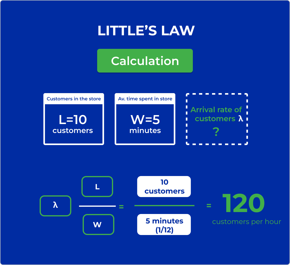
Little’s Law Example of a Bakery Queue
We’ll take the following example of a bakery shop queue. Consider a bakery where customers form a line to order and pick up their bagels. Let's assume the following for a particular hour:
- On average, 10 customers are in the shop (either waiting in line or waiting for their bagel sandwiches to be made).
- The average time a customer spends in the bakery, from entering the line to receiving their order, is 5 minutes.
Using Little's law, we can calculate the arrival rate of customers (λ):
Given L=10 customers and W=5 minutes (or 1/12 hour, since there are 60 minutes in an hour), we have:
λ=L/W=10 divided by 1/12=120 customers per hour
This means, on average, 120 customers visit the bakery each hour. Little's law helps understand the flow of customers and can aid in making decisions like staffing levels or the need for additional service counters to reduce waste, such as wait times.
Little's Law example
Little’s Law in Project Management
Regardless of its origins, Little’s law applies to a wide range of systems and approaches, including managing projects and workflows.
In such an environment, the law takes a slightly different approach. Instead of taking the arrival rate, it’s expressed by the departure rate of the system if we assume that the average arrival and departure rates are equal. For example, in a workflow management method such as kanban, the departure rate is known as “throughput”.
Speaking about kanban, one of its 6 core practices is limiting the work in progress to ensure a manageable number of active items are in progress at a given time. This helps keep the arrival and departure of work in the system stable.
In that context, the law is formulated as:
WIP = Throughput * Cycle Time
- WIP = the number of work items in progress
- Throughput = the number of completed work items
- Cycle time = the time for processing the work items
The main goal here is to unlock predictability by keeping a stable flow of work so that you can be more confident when communicating commitments with your customers.
Apart from having the average arrival rate match the average departure rate, there are a few more assumptions that Little’s law makes. Let’s take a look at them below.
- Everything that enters the system will eventually leave it.
- WIP shouldn't vary greatly between the beginning and the end of the analyzed time period.
- The average WIP age should neither be increasing nor decreasing.
- Cycle Time, Work In Progress, and Throughput should be measured using consistent units.
What Is the Importance of Little's Law in Flow Management?
Little’s law can be an invaluable tool for analyzing and optimizing various queuing systems.
But what truly makes the famous equation extremely powerful is its ability to help managers create a highly predictable process. This is not to say that Little’s law should be applied for meticulous forecasts, as the formula is based on averages. Instead, it helps build a system that operates according to your expectations. In such a predictable environment, Little’s law can aid in setting up SLEs - service level expectations with other teams or third parties.
To quote the flow expert, Mr. Daniel Vacanti: "if you know how flow works, then you know how value delivery works."
What Are Little’s Law Benefits?
As discussed, Little's law is widely applicable across various fields and systems, providing several valuable benefits. Here are three of the most significant advantages:
-
Simplicity and Universality: Little’s law doesn't rely on specific distribution types for arrival or service times. It is applicable in various scenarios, from manufacturing to retail, healthcare, and even computer networks. This universality makes it a powerful tool for analysts and managers who need a straightforward understanding of system behavior without delving into complex statistical models.
-
Performance Measurement and Improvement: Little's law provides a straightforward means to measure and improve the performance of a system. By understanding the relationship between the number of items in the system, the arrival or throughput rates, and the time spent in the system, managers can identify bottlenecks and inefficiencies.
-
Process Predictability: Little’s law offers an in-depth understanding of the arrival and exit rate of work items into the system. By doing so, it supports improvement on the basis of stable processes and enables more accurate forecasting. Understanding the throughput of a team, for instance, is a key indicator of the team's delivery capabilities. Furthermore, applying work-in-progress limits helps level the system so that you can match arrivals with departures.
As can be seen, Little's law has numerous advantages. It is a valuable tool for project managers aspiring to optimize their project delivery through better flow management and continuous improvement of processes.
Little’s Law Frequently Asked Questions (FAQs)
What Is Flow Time?
In Lean, "flow time," or "lead time" refers to the total time it takes for a product or service to pass through the entire process or system, from the initial step to the final output. This includes not only the actual processing time but also any time spent waiting between steps, moving from one process to another including quality checks or inspections.
What Are Flow Metrics?
In Lean/Agile management, flow metrics provide a clear understanding of how work gets done and the foundation to create a stable workflow. The most important flow metrics include cycle time, lead time, throughput, and work in progress.
What’s the Formula for Little’s Law in Kanban?
In the context of kanban, a popular method for managing and improving work across systems, Little's law is applied to help teams understand and manage their workflow more effectively. The formula remains fundamentally the same but is expressed slightly differently to emphasize departure (throughput) instead of arrival rate.
Average Work in Progress (WIP)=Throughput × Average Cycle Time
We offer the most flexible software platform
for outcome-driven enterprise agility.
In Summary
Little’s law is a fundamental equation in queuing theory that describes the relationship between the average number of work items in a system, their arrival rate, and the time they spend in the process. The formula is L=λW, where L indicates the average number of items in the system, λ - is the average number of items arriving at the system per unit of time, and W - is the average waiting time an item spends in a queuing system.
Thanks to its simplicity, Little’s law is successfully applied for:
- Performance measurement
- Continuous improvement
- Process predictability